Betadisper Distances Plotted Against Continuous Data
Takes the output of dist_calc function. Or use with the result of the permanova function to ensure the results correspond to exactly the same input data. Runs betadisper for all categorical variables in variables argument. See help('betadisper', package = 'vegan').
dist_bdisp ( data, variables, method = c ( "centroid", "median" ) [[ 1 ] ], complete_cases = TRUE, verbose = TRUE ) Arguments
- data
-
ps_extra output from dist_calc
- variables
-
list of variables to use as group
- method
-
centroid or median
- complete_cases
-
drop samples with NAs in any of the variables listed
- verbose
-
sends messages about progress if true
Value
ps_extra list containing betadisper results
Examples
library ( phyloseq ) library ( vegan ) #> Loading required package: permute #> Loading required package: lattice #> This is vegan 2.6-4 data ( "dietswap", package = "microbiome" ) # add some missings to demonstrate automated removal sample_data ( dietswap ) $ sex [ 3 : 6 ] <- NA # create a numeric variable to show it will be skipped with a warning dietswap <- ps_mutate ( dietswap, timepoint = as.numeric ( timepoint ) ) # straight to the betadisp bd1 <- dietswap %>% tax_agg ( "Genus" ) %>% dist_calc ( "aitchison" ) %>% dist_bdisp (variables = c ( "sex", "bmi_group", "timepoint" ) ) %>% bdisp_get ( ) #> Dropping samples with missings: 4 #> Warning: Variable 'timepoint' is skipped as it cannot be used for grouping (class = 'numeric') bd1 $ sex #> $model #> #> Homogeneity of multivariate dispersions #> #> Call: vegan::betadisper(d = distMat, group = meta[[V]], type = method) #> #> No. of Positive Eigenvalues: 123 #> No. of Negative Eigenvalues: 0 #> #> Average distance to centroid: #> female male #> 10.022 9.059 #> #> Eigenvalues for PCoA axes: #> (Showing 8 of 123 eigenvalues) #> PCoA1 PCoA2 PCoA3 PCoA4 PCoA5 PCoA6 PCoA7 PCoA8 #> 5106.7 2075.2 1360.1 1281.4 1061.7 890.1 665.4 567.5 #> #> $anova #> Analysis of Variance Table #> #> Response: Distances #> Df Sum Sq Mean Sq F value Pr(>F) #> Groups 1 50.14 50.144 20.976 7.853e-06 *** #> Residuals 216 516.35 2.391 #> --- #> Signif. codes: 0 '***' 0.001 '**' 0.01 '*' 0.05 '.' 0.1 ' ' 1 #> #> $tukeyHSD #> Tukey multiple comparisons of means #> 95% family-wise confidence level #> #> Fit: aov(formula = distances ~ group, data = df) #> #> $group #> diff lwr upr p adj #> male-female -0.9632687 -1.377813 -0.5487242 7.9e-06 #> #> # quick vegan plotting methods plot ( bd1 $ sex $ model, label.cex = 0.5 ) 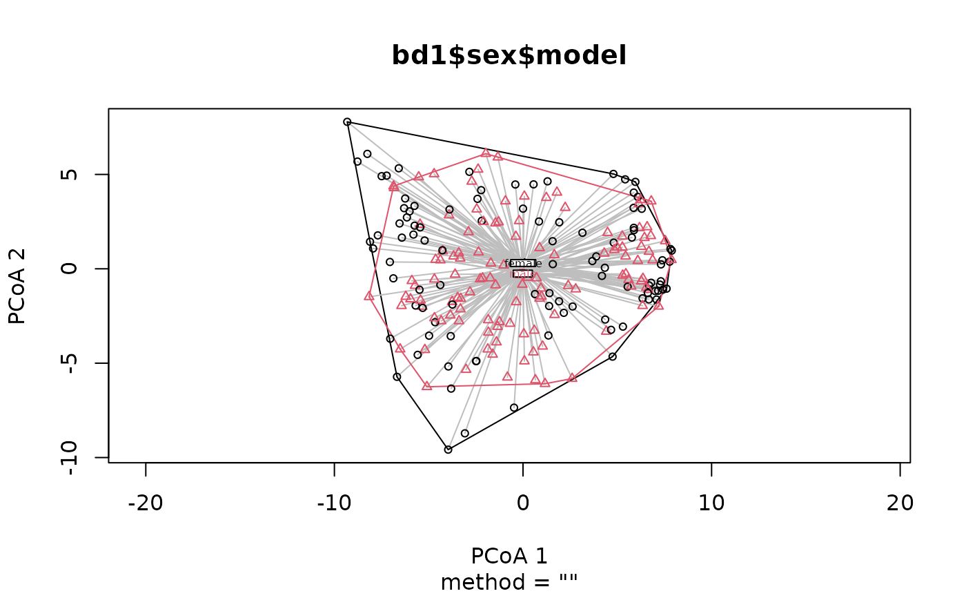 boxplot ( bd1 $ sex $ model )
 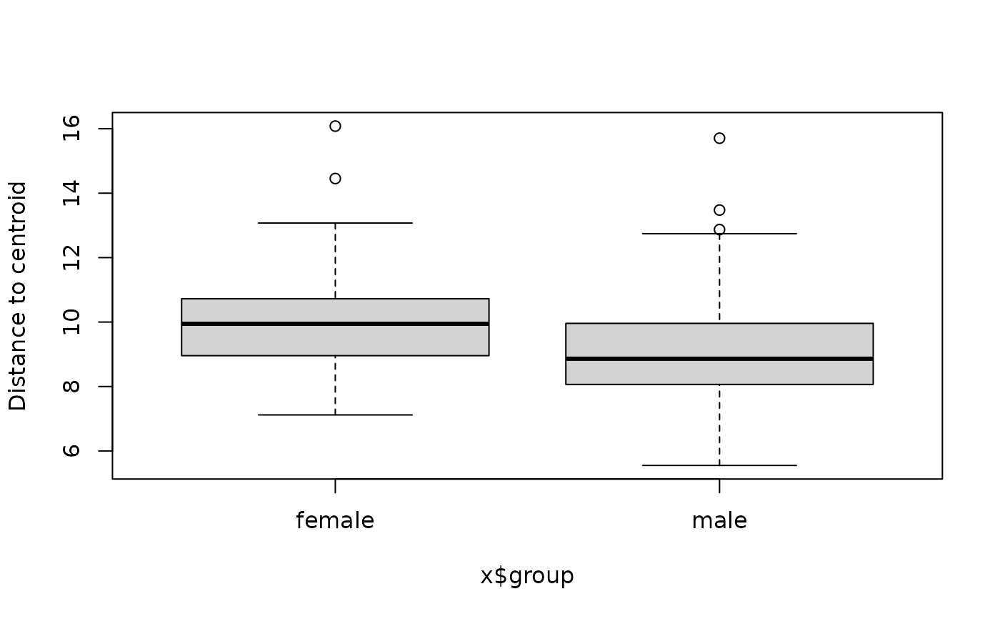 # compute distance and use for both permanova and dist_bdisp testDist <- dietswap %>% tax_agg ( "Genus" ) %>% dist_calc ( "bray" ) PERM <- testDist %>% dist_permanova ( variables = c ( "sex", "bmi_group" ), n_processes = 1, n_perms = 99 ) #> Dropping samples with missings: 4 #> 2022-10-20 20:40:36 - Starting PERMANOVA with 99 perms with 1 processes #> 2022-10-20 20:40:36 - Finished PERMANOVA str ( PERM, max.level = 1 ) #> List of 5 #> $ ps :Formal class 'phyloseq' [package "phyloseq"] with 5 slots #> $ dist : 'dist' num [1:23653] 0.764 0.731 0.728 0.664 0.744 ... #> ..- attr(*, "Labels")= chr [1:218] "Sample-1" "Sample-2" "Sample-7" "Sample-8" ... #> ..- attr(*, "Size")= int 218 #> ..- attr(*, "call")= language as.dist.default(m = as.matrix(distMat)[keepers, keepers]) #> ..- attr(*, "Diag")= logi FALSE #> ..- attr(*, "Upper")= logi FALSE #> $ ord : NULL #> $ info : 'ps_extra_info' Named chr [1:7] "Genus" NA NA "bray" ... #> ..- attr(*, "names")= chr [1:7] "tax_agg" "tax_transform" "tax_scale" "distMethod" ... #> $ permanova:Classes 'anova.cca', 'anova' and 'data.frame': 4 obs. of 5 variables: #> ..- attr(*, "heading")= chr [1:2] "Permutation test for adonis under reduced model\nMarginal effects of terms\nPermutation: free\nNumber of permutations: 99\n" "vegan::adonis2(formula = formula, data = metadata, permutations = n_perms, by = by, parallel = parall)" #> ..- attr(*, "F.perm")= num [1:99, 1:2] 2.596 0.417 0.917 1.38 2.706 ... #> ..- attr(*, "Random.seed")= int [1:626] 10403 30 515190382 2133433928 917665867 1283494313 1101294840 1366013990 -351622847 676521683 ... #> ..- attr(*, "control")=List of 12 #> .. ..- attr(*, "class")= chr "how" #> - attr(*, "class")= chr [1:2] "ps_extra" "list" bd <- PERM %>% dist_bdisp (variables = c ( "sex", "bmi_group" ) ) bd #> ps_extra object - a list with phyloseq and extras: #> #> phyloseq-class experiment-level object #> otu_table() OTU Table: [ 130 taxa and 218 samples ] #> sample_data() Sample Data: [ 218 samples by 8 sample variables ] #> tax_table() Taxonomy Table: [ 130 taxa by 3 taxonomic ranks ] #> #> ps_extra info: #> tax_agg = Genus tax_transform = NA #> #> bray distance matrix of size 218 #> 0.7639533 0.731024 0.7283254 0.6637252 0.7437293 ... #> #> permanova: #> Permutation test for adonis under reduced model #> Marginal effects of terms #> Permutation: free #> Number of permutations: 99 #> #> vegan::adonis2(formula = formula, data = metadata, permutations = n_perms, by = by, parallel = parall) #> Df SumOfSqs R2 F Pr(>F) #> sex 1 0.361 0.00933 2.1539 0.17 #> bmi_group 2 2.377 0.06143 7.0888 0.01 ** #> Residual 214 35.874 0.92720 #> Total 217 38.691 1.00000 #> --- #> Signif. codes: 0 '***' 0.001 '**' 0.01 '*' 0.05 '.' 0.1 ' ' 1 #> #> #> betadisper: #> sex bmi_group
 chowarorinced1959.blogspot.com
Source: https://david-barnett.github.io/microViz/reference/dist_bdisp.html
0 Response to "Betadisper Distances Plotted Against Continuous Data"
Postar um comentário